GP-SUM
Suddhu | June 16th 2020, RPL reading group | paper link
Overview
- Captures complex belief distributions and noisy dynamics
- System where multimodality and complex behaviors cannot be neglected, at the cost of larger computational effort
- GP-SUM comprises of:
- Dynamic models expressed as a GP
- Complex state represented as weighted sum of Gaussians
- Can be viewed as both a sampling technique and a parametric filter
- Applications: (i) synthetic benchmark task, (ii) planar pushing
1. Introduction
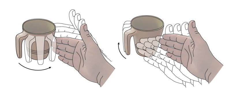
- Cases where state belief cannot be approximated as a unimodal Gaussian distribution
- Example: push grasping (Dogar and Srinivasa)
- Theoretical contribution: Bayes updates of belief without linearization, or unimodal Gaussian approximation
2. Related work
- Gaussian processes have been applied to learn dynamics models, planning/control, system identification, and filtering.
- GP-Bayes filters learn dynamics and measurement models:
- GP-EKF: linearizes GP model to guarantee final Gaussian (Ko and Fox)
- GP-UKF: similar to the unscented Kalman filter (Ko and Fox)
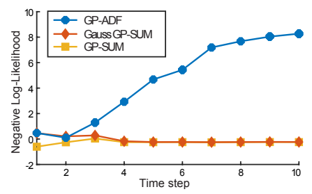
- GP-ADF: computes first two moments and returns Gaussian (Deisenroth and Hanebeck)
- GP-PF: no closed form distributions, particle depletion (Ko and Fox)
- Task-specific:
- MHT: multi-hypothesis tracking, joint distribution as a Gaussian mixture (Blackman)
- MPF: manifold particle filter, sampling-based algorithm to decompose state space using contacts (Koval)
3. Background on GP filtering
3.1 Bayes filters
- Track the state of system
x_tprobabilistically:- action
u_(t-1)evolves state fromx_(t-1)tox_t
- Observation
z_toccurs
- Belief:
- action
- Two steps: prediction update and measurement update
3.1.1 Prediction update
- given system dynamics and previous belief, we compute prediction belief:

- Integral cannot be solved analytically: linearize dynamics and assume Gaussian distribution (EKF)
3.1.2 Measurement update
- Given prediction belief and new measurement
z_twe recover belief: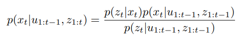
Equation 2
- For closed form: linearize observation model and assume Gaussian
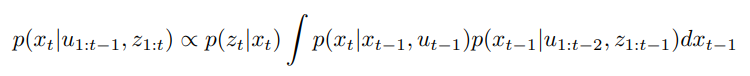
3.1.3 Recursive belief update
- Combine Equation 1 and Equation 2 to express belief with respect to previous belief, dynamic model and observation model:
3.2 Gaussian processes
- Real systems may have unknown or inaccurate models, can be learnt via GPs
- Advantages:
- Learns high-fidelity model from noisy data
- Estimates uncertainty of predictions from data (ie: quality of regression)
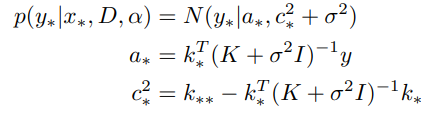
- Output and latent function:
- We need data and kernel function:
- Mean and variance equations (kernel: square exponential):
4. GP-SUM Bayes filter
- Dynamics model
p(x_t | x_(t-1), u_(t-1))and measurement modelp(z_t | x_t)are represented by GP
- Considers the weak assumption that belief is approximated by sum of Gaussians
- at infinite samples this converges to the real distribution
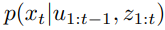
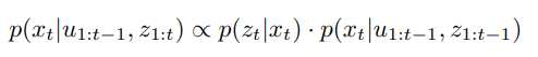
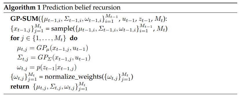
4.1 Updating the prediction belief
- Belief from standard Bayes filter:
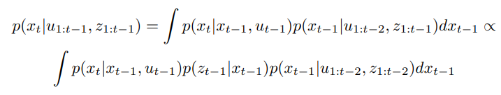
- Prediction belief (combining Equation 1 and Equation 5):
- updated with previous prediction belief, dynamics model, and observation model
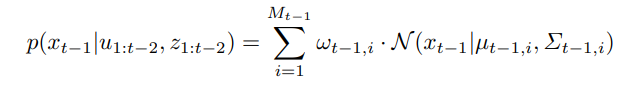
- Prediction belief at
(t-1)approximated as sum of GaussiansM_(t - 1)# of components andw_(t - 1), iweight of Gaussian mixture
- Sampling from this distribution, we can simplify Equation 7 as:
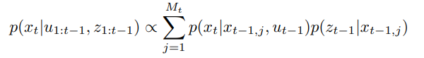
- Dynamics model can be expressed as Gaussian (GP):
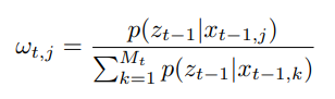
- Weight depends on the observations:
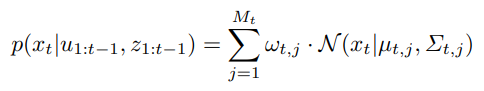
- Final prediction belief:
- Other GP-Bayes filters approximate the prediction belief as a single Gaussian, and previous approximation accumulate over time
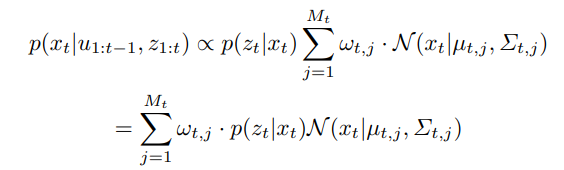
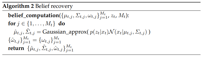
4.2 Recovering belief from prediction belief
- From Equation 5 and Equation 10, the belief is a sum of Gaussians:
p(z_t | x_t) N(x_t | mu_t, j, Sigma_t, j)won't be proportional to a Gaussian, so they recover belief through an approximation (Deisenroth and Hanebeck)- won't go into detail but preserves the first two moments of
p(z_t | x_t) N(x_t | mu_t, j, Sigma_t, j)
- only needed to recover belief, does not accumulate as iterative filtering error
- won't go into detail but preserves the first two moments of
4.3 Computational complexity
- GP-SUM complexity increases linearly with # of Gaussians sampled
M
- Also depends on size of GP model
n
- cost of propagating prediction belief:
5. Results
5.1 1D non-linear synthetic model
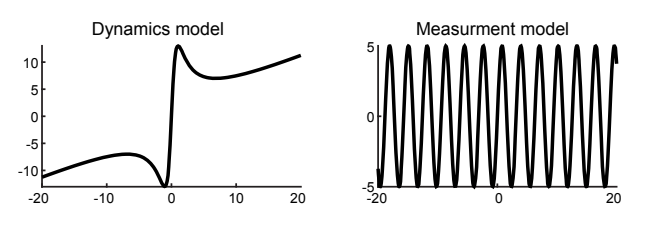
Dynamics model (especially sensitive around 0):
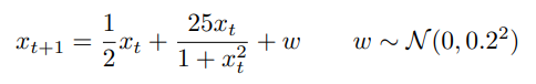
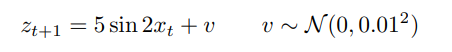
Measurement model:
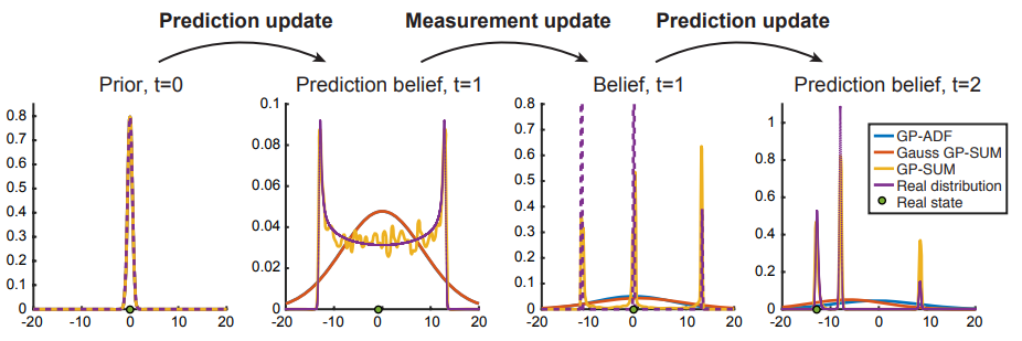
t = 2 while other methods output a single Gaussian to enclose them
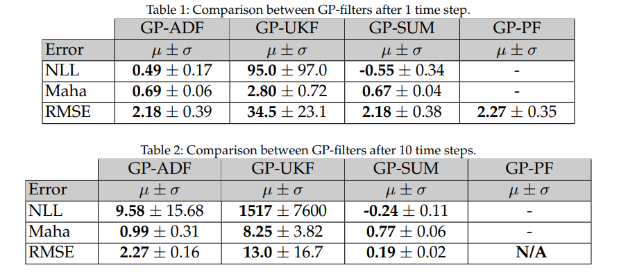
t = 1, GP-SUM shows better metrics across all 3. GP-PF becomes particle starved soon at t = 10
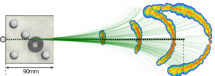
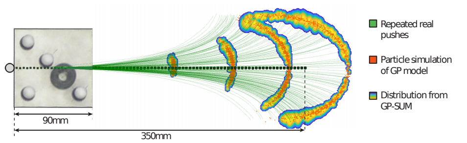
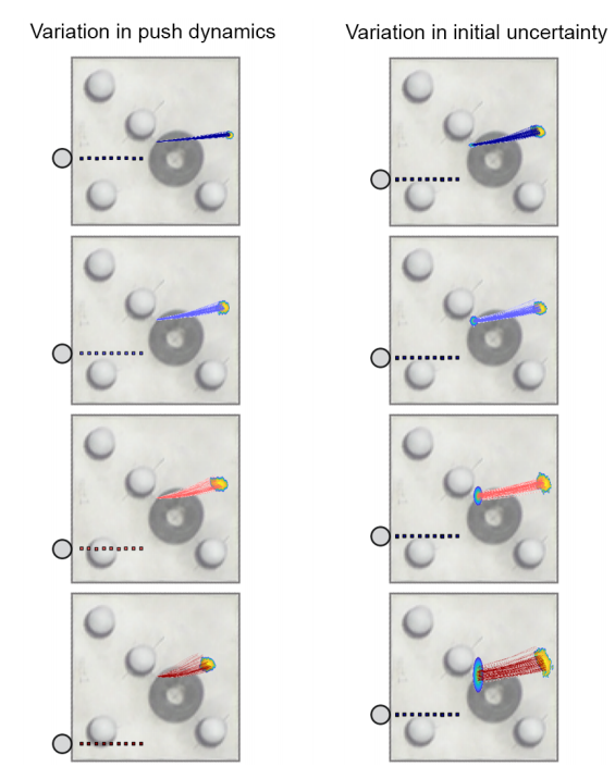
5.2 Real task: uncertainty in pushing
- Planar pushing yields stochastic behavior due to friction variability and uncertain interactions
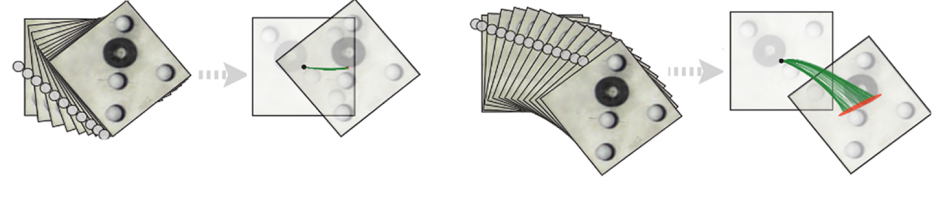
- Heteroscedastic: noise in pushing dynamics depends on the action
- Use GP-SUM to propagate uncertainty in planar pushing by learning the dynamics of system with a heteroscedastic GP (Bauza and Rodriguez)
- train GP:
- input =
contact_points, pusher_velocity, pusher_direction
- output =
object_displacement
- input =
- train GP:
- Notable difference, there is no measurement model. State distribution can only expand over time, and weights are equal.
- Propagating uncertainty of pushing can:
- inform strategies that reduce uncertainty (active)
- better perform pose estimation
6. Discussion and future work
- Situations where Gaussian beliefs are unreasonable
- Future work:
- # of samples: adjusting over time (particle filter methods)
- computational cost: scale linearly with # of samples.
- GP extensions: can use sparse GPs (Pan and Boots)